Continuing from Part 1 of this series, intuitively, one could expect that the resonant tire frequency in the data would change with changes in vehicle speed. The slower the speed, the lower the resonant frequency – the faster the speed, the higher the resonant frequency. This begged the question, could I link this kind of frequency response to specific vehicle tires? If so, then we might have the ability to identify, and predict when tires are either approaching, or at the point of imbalance, based upon their frequency and comparable amplitude (lateral to vertical amplitudes).
For my measurement effort, I noted my vehicle’s tires had a loaded diameter (ground to top of tire) of 29”. Knowing that a tire’s circumference can be calculated using the formula C = 2πr, that means it travels 91” during every full rotation. For a given vehicle speed, we can calculate the number of tire rotations per second, which can then be described in terms of frequency/Hz./cycles per second. Click on the image below to see an animation of how tire radius/diameter, vehicle speed and tire resonant frequency can be associated.
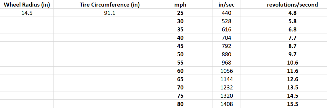
The table below highlights several different vehicle speeds and the calculated frequency response I would expect to see from my vehicle tires.
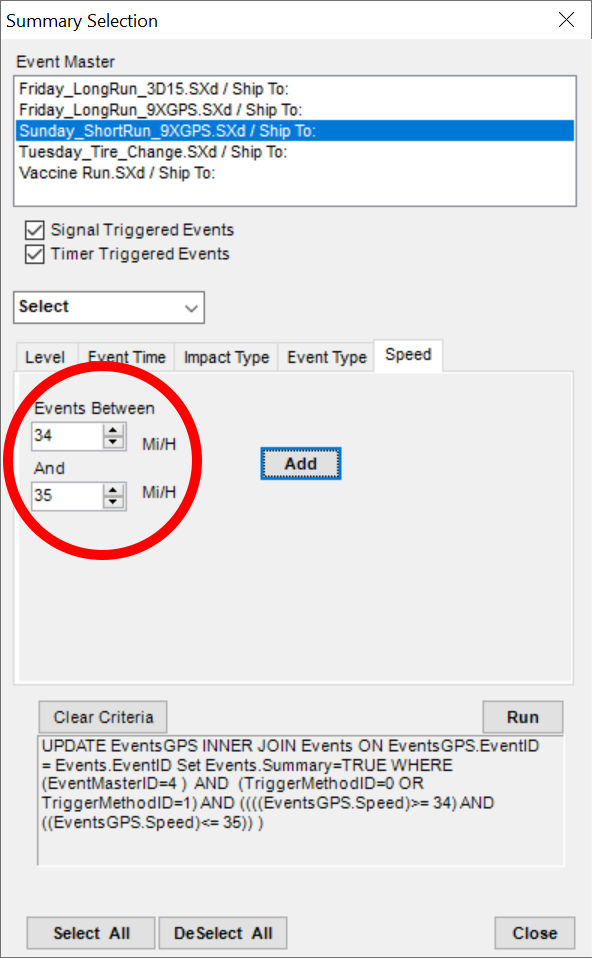
Since I used a SAVER 9XGPS for my measurement, I had the accompanying GPS information for each captured time-domain event, which includes my vehicle speed. I used SaverXware's smart event summary selection criterion, selecting only those time-domain events that were captured when my vehicle was traveling at a specific speed, or within a tight range of speeds. Using the table as a guide above, I selected only those events when my vehicle was traveling around 35 mph.
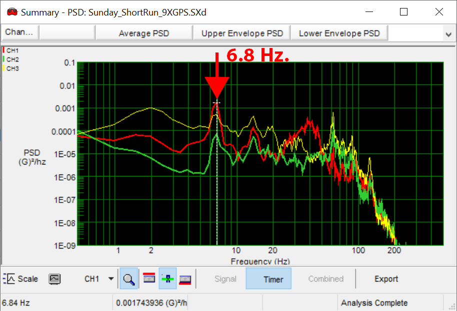
With that selection, my table indicates I should then generate a Summary PSD that shows a prominent tire resonance at around 6.8 Hz. In fact, my summary PSD (shown below) showed precisely that information. Additionally, that PSD communicates that the lateral side-to-side motion at that frequency was greater than the vertical motion, which helps explain why the bottles would be clanking together so prominently/noticeably.
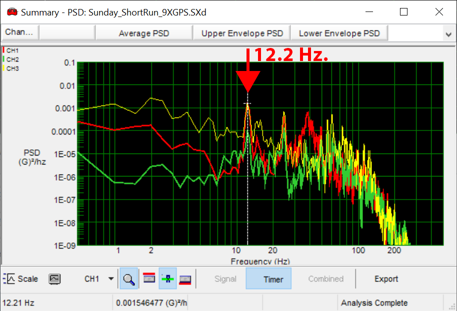
If I want to see what the response looks like at highway speeds, I can use my SaverXware Summary Selector to choose those events where I was traveling between 64-65 mph. At that speed, I would expect to see a tire resonance at about 12.5 Hz. In fact, once again, the summary PSD below shows precisely that information. At this vehicle speed, the tire resonant response is similar in both lateral and vertical amplitude.
If I consider a summary of all the events recorded during my 15-mile loop, those events obviously were captured at different vehicles speeds, so it might seem a bit more challenging to see the evidence, or signature of those resonant tire frequencies in one all-inclusive summary PSD plot.
However, realistic cargo transport occurs with vehicle speeds in a predictable speed range – on the low-end, maybe 30 mph in city/local areas, and on the high-end, maybe 65-70 mph. For my loop, my vehicle speed range was more in the 30-75 mph range. Though that might seems like a fairly large range, in-terms of corresponding tire resonant frequency range, it’s quite narrow.
Using the table above, a 30-75 mph range would correspond to a frequency bandwidth of about 6.0 – 14.5 Hz. After generating a summary PSD using all my captured events, it’s evident there is a fair amount of both lateral and vertical input within that 6 – 14 Hz. range – which indicates my car was wobbling at all speeds ranging from 30-75 mph.
We can use a unique SaverXware ETC filtering capability (cutoff filter) to allow us to focus on just that tight frequency range that occurs in a certain bandwidth, say 5-18 Hz., which helps to “see” the frequency content of interest more clearly, while removing potentially distracting frequency content from the view. After applying that cutoff filter, the single event PSD below shows how we can focus our view within that bandwidth of interest.
The clear resonant frequency of 14.6 Hz. means that I was traveling 75 mph when that event was captured - and once again, the lateral input to my vehicle was equivalent to the vertical input at that frequency.
By creating an animation of a section of travel, where I entered onto a freeway, accelerated to speed, and eventually exited off, you can clearly see the changes in tire frequency as my car changed speeds. Click the image below to see the animation.
[video width="1322" height="1080" mp4="/wp-content/uploads/2021/10/Speed-Tire-Frequency-Change.mp4" poster="/wp-content/uploads/2021/10/Tire-Frequency-Video-Thumbnail3.png"][/video]
In the next email, we’ll highlight the differences in vibration signatures after replacing the old tires with new ones.
Continuing from Part 1 of this series, intuitively, one could expect that the resonant tire frequency in the data would change with changes in vehicle speed.
The slower the speed, the lower the resonant frequency – the faster the speed, the higher the resonant frequency. This begged the question, could I link this kind of frequency response to specific vehicle tires?
If so, then we might have the ability to identify, and predict when tires are either approaching, or at the point of imbalance, based upon their frequency and comparable amplitude (lateral to vertical amplitudes).
For my measurement effort, I noted my vehicle’s tires had a loaded diameter (ground to top of tire) of 29”. Knowing that a tire’s circumference can be calculated using the formula C = 2πr, that means it travels 91” during every full rotation. For a given vehicle speed, we can calculate the number of tire rotations per second, which can then be described in terms of frequency/Hz./cycles per second.
Click on the image below to see an animation of how tire radius/diameter, vehicle speed and tire resonant frequency can be associated.
The table below highlights several different vehicle speeds and the calculated frequency response I would expect to see from my vehicle tires.
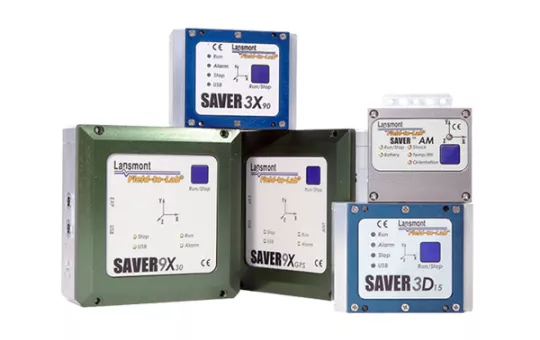
Since I used a SAVER 9XGPS for my measurement, I had the accompanying GPS information for each captured time-domain event, which includes my vehicle speed.
I used SaverXware's smart event summary selection criterion, selecting only those time-domain events that were captured when my vehicle was traveling at a specific speed, or within a tight range of speeds.
Using the table as a guide above, I selected only those events when my vehicle was traveling around 35 mph.
With that selection, my table indicates I should then generate a Summary PSD that shows a prominent tire resonance at around 6.8 Hz. In fact, my summary PSD (shown below) showed precisely that information.
Additionally, that PSD communicates that the lateral side-to-side motion at that frequency was greater than the vertical motion, which helps explain why the bottles would be clanking together so prominently/noticeably.
If I want to see what the response looks like at highway speeds, I can use my SaverXware Summary Selector to choose those events where I was traveling between 64-65 mph.
At that speed, I would expect to see a tire resonance at about 12.5 Hz. In fact, once again, the summary PSD below shows precisely that information.
At this vehicle speed, the tire resonant response is similar in both lateral and vertical amplitude.
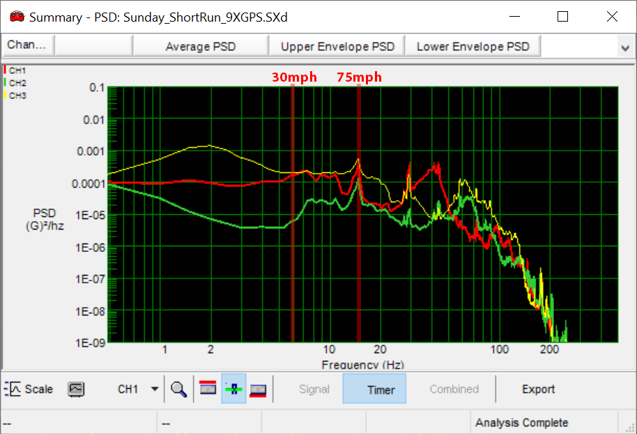
If I consider a summary of all the events recorded during my 15-mile loop, those events obviously were captured at different vehicles speeds, so it might seem a bit more challenging to see the evidence, or signature of those resonant tire frequencies in one all-inclusive summary PSD plot.
However, realistic cargo transport occurs with vehicle speeds in a predictable speed range – on the low-end, maybe 30 mph in city/local areas, and on the high-end, maybe 65-70 mph.
For my loop, my vehicle speed range was more in the 30-75 mph range. Though that might seems like a fairly large range, in-terms of corresponding tire resonant frequency range, it’s quite narrow. Using the table above, a 30-75 mph range would correspond to a frequency bandwidth of about 6.0 – 14.5 Hz.
After generating a summary PSD using all my captured events, it’s evident there is a fair amount of both lateral and vertical input within that 6 – 14 Hz. range – which indicates my car was wobbling at all speeds ranging from 30-75 mph.
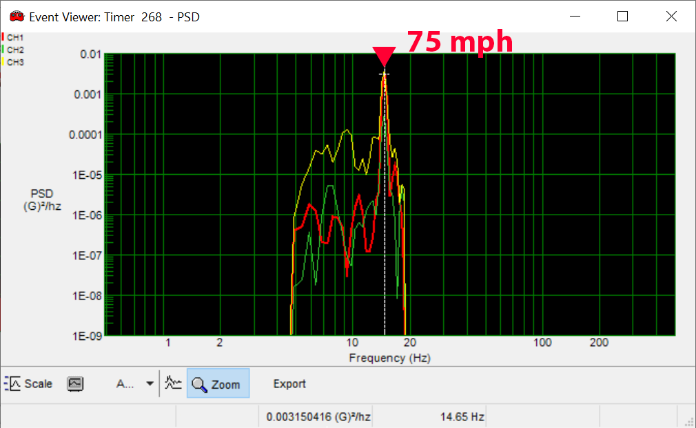
We can use a unique SaverXware ETC filtering capability (cutoff filter) to allow us to focus on just that tight frequency range that occurs in a certain bandwidth, say 5-18 Hz., which helps to “see” the frequency content of interest more clearly, while removing potentially distracting frequency content from the view.
After applying that cutoff filter, the single event PSD below shows how we can focus our view within that bandwidth of interest. The clear resonant frequency of 14.6 Hz. means that I was traveling 75 mph when that event was captured - and once again, the lateral input to my vehicle was equivalent to the vertical input at that frequency.
By creating an animation of a section of travel, where I entered onto a freeway, accelerated to speed, and eventually exited off, you can clearly see the changes in tire frequency as my car changed speeds.
Click the image below to see the animation.